Ch 8: Regression models for Quantitative and Qualitative predictors

Outline

1. Polynomial regression
2. Interaction regression models
3. Qualitative predictors
   • Use of indicator (dummy) variables
   • Use of allocated variables

---

1. Polynomial regression

When the response function is indeed a polynomial function, we can easily fit polynomial regression by LSE. Second-order polynomial regression with one-variable can be written as

\[Y_i = \beta_0 + \beta_1 x_i + \beta_2 x_i^2 + \epsilon_i\]

where \(x_i = X_i - \bar{X}\).

Note We use centered predictor variables because in the polynomial regression model, \(X\) and \(X^2\) often will be highly correlated. This, as we noted in Ch 7, can cause serious computational difficulties. Centering the predictor variable often reduces the multicollinearity substantially.

drawbacks

1. hard to interprete
2. poor prediction
3. predictor variables are likely to have multicollinearity

2. Interaction regression models

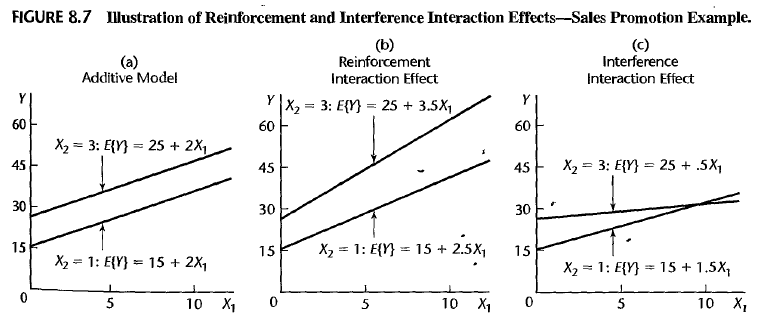
Here we have a regression model with interaction term \(X_1X_2\).

\[Y_i = \beta_0 + \beta_1 X_{i1} + \beta_2 X_{i2} + \beta_3 X_{i1}X_{i2} + \epsilon_i\]

where \(E(Y_i) = \beta_0 + \beta_1 X_{i1} + \beta_2 X_{i2} + \beta_3 X_{i1}X_{i2}\).

interpretation

1. The change in mean response when \(X_{i1}\) changes one unit (\(\Delta X_{i1} = 1\)) where \(X_{i2}\) is fixed : \(\beta_0 + \beta_3 X_{i2}\)
2. Assuming that \(\beta_1>0, \beta_2>0\),
   \(\beta_3>0\) implies reinforcement (synergetic)
   \(\beta_3<0\) implies interference (antagonistic)

3. Qualitative predictors

Classification of qualitative variables

• nominal variables (ex) gender, disability, bloodtype
• ordinal (ex) grade

When we want to analyze a regression model by several categories, a good way is to add qualitative variables indicating different classes. Let’s figure out how to put these variables in regression model, and how to interprete the result.

Use of indicator (dummy) variables

A dummy variable \(X_k\) indicates 1 as true or 0 as false. It could be used to encode nomial variables with several classes/categories.

When we are given \(c\) different categories, then how many dummy variables should we add in the model?

Case 1 2 classes (stock company / mutual company), 2 dummy variables

• \(X_2 = 1\) if stock company and \(X_2 = 0\) otherwise.
• \(X_3 = 1\) if mutual company and \(X_3 = 0\) otherwise. \(\Rightarrow Y_i = \beta_0 + \beta_1 X_{i1} + \beta_2 X_{i2} + \beta_3 X_{i3} + \epsilon_i\) Then the design matrix \(X\) is \([1, X_{11}, 1, 0 ; 1, X_{11}, 1, 0 ; 1, X_{11}, 0, 1 ; 1, X_{11}, 0, 1 ; \cdots ; 1, X_{11}, 1, 0]\)

Note that the 1, 3, 4 columns are linearly dependent. \(X_0 = X_2 + X_3\). This leads to the matrix \(X^tX\) to be rank defficient (\(det(X^tX)=0\)).

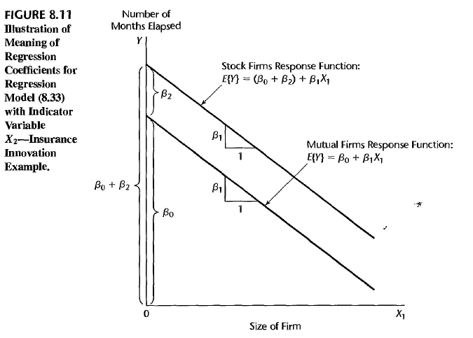
Case 2 2 classes (stock company / mutual company), 1 dummy variable

• \(X_2 = 1\) if stock company and \(X_2 = 0\) otherwise (mutual company). \(\Rightarrow Y_i = \beta_0 + \beta_1 X_{i1} + \beta_2 X_{i2} + \epsilon_i\) You can expect that the design matrix \(X\) is the same as above except for the last column. Now 3 columns are linearly independent.

The response function is given as

• \(E(Y) = \beta_0 + \beta_2 + \beta_1 X_{1}\) for stock company, and
• \(E(Y) = \beta_0 + \beta_1 X_{1}\) for mutual company.

These two categories can be drawn as different lines which has the same slope but different intercept.

Case 3 3 classes (stock company / mutual company / international company), 2 dummy variables

• \(X_2 = 1\) if stock company and \(X_2 = 0\) otherwise.
• \(X_3 = 1\) if mutual company and \(X_3 = 0\) otherwise. \(\Rightarrow Y_i = \beta_0 + \beta_1 X_{i1} + \beta_2 X_{i2} + \beta_3 X_{i3} + \epsilon_i\) The columns of the design matrix \(X\) are linearly independent.

The response function is given as

• \(E(Y) = \beta_0 + \beta_2 + \beta_1 X_{1}\) for stock company,
• \(E(Y) = \beta_0 + \beta_3 + \beta_1 X_{1}\) for mutual company, and
• \(E(Y) = \beta_0 + \beta_1 X_{1}\) for international company.

These three categories can be drawn as three different lines which has the same slope but different intercepts.

Now we can summarize up that encoding \(c\) classes needs \(c-1\) dummy variables.

Use of allocated variables

An allocated variable \(X_k\) allots distinct integer numbers to different levels. It could be used to encode ordinal variables with several levels.

Note But you should make sure that the difference between each two factors are as much as the difference between allocated codes. Also you often use reference level as a baseline to compare the difference between levels. (ex) We have alphabetical grades as a ordinal variable. Take \(F\) level as baseline, and then you can compare the result between other levels by its difference between the baseline.

---

Here is the Jupyter notebook script to run several practice codes using R.