Ch 4: Diagnostics and Remedial Measures

Checklist to see if the linear model is appropriate

1. linearity
2. homogeneity (constant variance)
3. independency
4. normality
5. outliers
6. omission of other predictor variables

We can observe above properties from visual methods. Now, we are going to find which plots are relevant to check these properties. Moreover, we learn how could we revise the components in a model when there is some disparity between the real data and the requirements.

Notation

• residual \(e_i=Y_i - \hat{Y_i}\)
• mean of residuals \(\bar{e} = \frac{\sum_i e_i}{n} = 0\)
• variance of residualss \(s^2 = \frac{\sum_i e_i^2}{n-2} = \frac{SSE}{n-2} = MSE\)
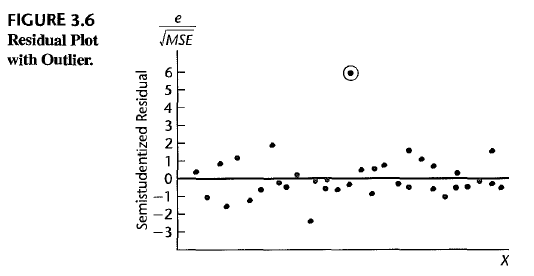
• semi-studentized residual \(e_i^\ast = \frac{e_i-\bar{e}}{\sqrt{MSE}} = \frac{e_i}{\sqrt{MSE}}\)

Outline

1. Graphical diagnostics
   • linearity
   • homogeneity
   • independency
   • normality
   • outliers
   • omission of other important predictors
2. Transformation of variables
   • Case 1: constant variance, but not-normal
   • Case 2: nonconstant variance and not-normal

---

1. Graphical diagnostics

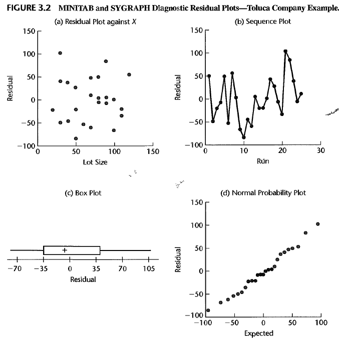
First, we identify useful plots.

linearity

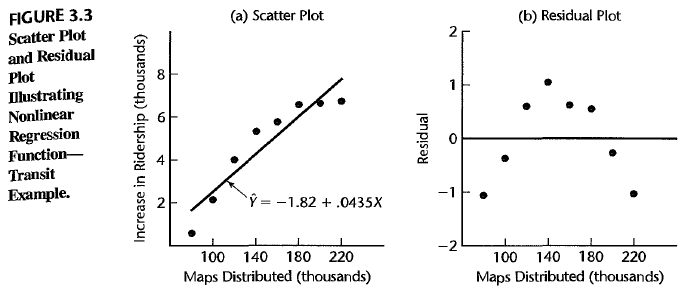
You can see a certain pattern. So, nonlinear!

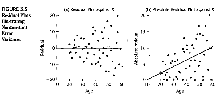
homogeneity

The errors should have the constant variance. i.e. \(\sigma^2(\epsilon_i) = const\). But if it isn’t, then you can also see the nonhomogeneous residuals.

independency

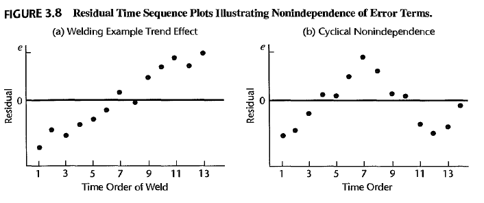
If \(corr(e_i,e_j) \neq 0\), then we can sse some systematic patterns.

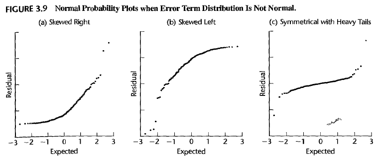
normality

You can check for the distribution by plotting a box plot, histogram, or Stem-and-Leaf plot. Or you can draw a normal Probability Plot.

outliers

You can draw a semi-standardized residual plot to figure out outliers.

omission of other important predictors

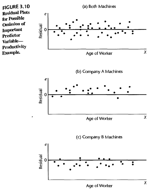
If some important predictors are omitted, the residuals may not be close to 0.

2. Transformation of variables

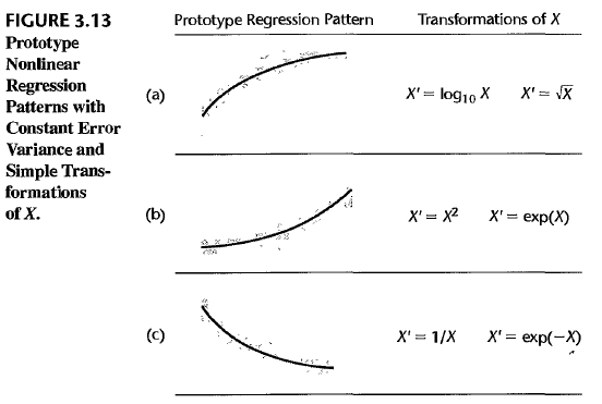
The basic idea is to linearize the variables by seeking the behavior of the error term.

Case 1: constant variance, but not-normal

Transform \(X\). Define a new variable as \(X^\prime = f(X)\) where \(f(\cdot)\) is a nonlinear function of \(X\), which could linearize the response \(Y\). Then use \(X^\prime\) instead of \(X\) in the linear model.

Case 2: nonconstant variance and not-normal

Transform \(Y\). Define a new variable as \(Y^\prime = g(Y)\) where \(g(\cdot)\) is a nonlinear function of \(Y\), which could linearize the response \(Y^\prime = f(X)\). Then use \(Y\prime\) instead of \(Y\) in the linear model. Transformation of \(Y\) modifies the variance of the responses, therefore right transformation could enable the data to have homogeneity.

Cf) Box-Cox transformation Transform \(Y\) by \(Y^\prime = Y^\lambda\) and identify the optimal \(\lambda \in \mathbb{R}\) by MLE or Least squares.