Ch 11: Remedial measures

Transformation is one of the standard remedial measure for a linear model. Recall that its uses are:

to linearize the regression relationship
to make the error distribution more nearly normal
to make the variances of the error terms more nearly equal.

In this chapter, we will find additional remedial measures to handle several pitfalls. Then we discuss non-parametric regression methods (which are quite different from previous regression models). A common feature of the remedial measures and alternative regression methods is that estimation procedures from the ways we’ve seen are relatively complex, so we need easier and more generic way to evaluate the precision of these complex estimators. Bootstrapping is one example.

Outline

Other remedial measures
- unequal error variance - weighted least squares
- multicollinearity - ridge regression
- influential cases - robust regression
Nonparametric regression
- regression trees
Bootstrap confidence intervals

1. Other remedial measures

unequal error variance - weighted least squares

Generalized multiple regression model $Y_i = \beta_0 + \beta_1 X_{i1} + \cdots + \beta_{p-1} X_{i,p-1} + \epsilon_i$ where $e_i$’s are independent, $e_i \sim N(0, \sigma_i^2)$, $$i = 1,2,\cdots, n

$. Here, the error variances may not be equal, so that$\sigma^2(\epsilon)$is an$n\times n$diagonal matrix where each entry has$\sigma_i^2$$.

When we use ordinary least square estimators, then still we have these properties:

the estimators of $\beta$ are unbiased
the estimators are consistent consistency is defined that $\forall \varepsilon >0, P(|b_n - \beta| \leq \varepsilon) = 1$ for succiciently large $n$ ($b_n$ converges to $\beta$). However, the estimators are no longer have minimum variance. This is due to the unequal error variances, making $n$ cases no longer have the same reliability. In other words, observations with small variances provide more reliable information.

A remedy to handle this problem is to use weighted least squares. First, we start from the simplest case.

when error variances are known Suppose that the errror variances $\sigma_i^2$ for all $n$ observations are given. Then we use Maximum likelihood method, again. First, we define the likelihood function $L(\beta)$.

\[L(\beta) = \prod_{i=1}^n \frac{1}{(2\pi \sigma_i^2)^\frac{1}{2}} exp [ - \frac{1}{2 \sigma_i^2} (Y_i - \beta_0 - \beta_1 X_{i1} - \cdots - \beta_{p-1} X_{i,p-1})^2 ]\]

Here, we substitute $w_i = \frac{1}{\sigma_i^2}$ and rewrite the formula.

\[L(\beta) = \prod_{i=1}^n \left( \frac{w_i}{2\pi}\right)^\frac{1}{2} exp [ - \frac{w_i}{2} (Y_i - \beta_0 - \beta_1 X_{i1} - \cdots - \beta_{p-1} X_{i,p-1})^2 ]\]

Since $\sigma_i^2$’s are known, parameters for likelihood function are just regression coefficients. Maximum likelihood method finds critical points which maximizes the likelihood function value.

This is just as the same as minimizing $Q_w = \sum_{i=1}^n w_i (Y_i - \beta_0 - \beta_1 X_{i1} - \cdots - \beta_{p-1} X_{i,p-1})^2$. The normal equation can be written using weights matrix $W = diag(w_1, w_2, \cdots, w_n)$ as below:

\[X^t WX b_w = X^tW Y\]

$\Rightarrow b_w = (X^t WX)^{-1} X^tW Y$ where $\sigma^2(b_w) = (X^t WX)^{-1}$. This is called Weighted least square estimator.

when variances are known up to proportionality constant Now, relaxing the condition, assume that we only know proportions among error variances. Consider a case that the second error variance is twice larger than the first one. i.e. $\sigma_2^2 = 2*\sigma_1^2$. Then we can write $w_i$’s in this form: $w_i = \frac{1}{k_i\sigma^2}$ where $\sigma^2$ is unknown true error variance of $\epsilon_1$. Then, $p \times p$ matrix $\sigma^2 (b_w) = \sigma^2 (X^t K X)^{-1}$, where $K = diag(k_1, k_2, \cdots, k_n)$. Since $\sigma^2$ is unknown, we use $s^(b_w) = MSE_w (X^t K X)^{-1}$, instead, where $MSE_w = \frac{\sum_{i=1}^n w_i (Y_i - \hat{Y_i})^2}{n-p} = \frac{\sum_{i=1}^n w_i e_i^2}{n-p}$.

when error variances are unknown We use estimators of the error variances. There are two approaches.

Estimation by residuals $\sigma_i^2 = E(\epsilon^2) - [E(\epsilon)]^2 = E(\epsilon^2)$. Hence, the squared residual $e_i^2$ is an estimator of $\sigma_i^2$.
Use of replicates or near replicates
- In a designed experiment (such as scientific simulations), replicate observations could be made. If the number of replicates is large, use the fact that sample variance gets closer to variance.
- However, in an observational studies (such as social studies), we use near observations as replicates.

Inference procedures should be followed when weights are estimated. We want to estimate a variance-covariance matrix $\sigma^2(b_w)$. The confidence intervals for regression coefficients are estimated with $s^2(b_{w_k})$ where $k$ stands for a bootstrap index. Then apply bootstraping method.

Lastly, we can use the ordinary least squares leaving the error variances unequal. Regression coefficient $b$ is still unbiased and consistent, but no longer a minimum variance estimator, where its variance is given as $\sigma^2(b) = (X^tX)^{-1} X^t \sigma^2(\epsilon)X (X^tX)^{-1}$ and it is estimated by $s^2(b) = (X^tX)^{-1} X^t S_0 X (X^tX)^{-1}$ where $S_0 = diag(e_1^2, e_2^2, \cdots, e_n^2)$.

Remark on weighted least squares Weighted least squares can be interpreted as transforming the data $(X_i, Y_i, \epsilon_i)$ by $W^{\frac{1}{2}}$. This can be written as

\[W^{\frac{1}{2}}Y = W^{\frac{1}{2}}X\beta + W^{\frac{1}{2}}\epsilon\]

and by setting $Y_w = W^{\frac{1}{2}} Y$, $X_w = W^{\frac{1}{2}} X$, and $\epsilon_w = W^{\frac{1}{2}} \epsilon$, the transformed variables follow the ordinary linear regression model

\[Y_w = X_w \beta + \epsilon_w\]

where $E(\epsilon_w) = W^{\frac{1}{2}} E(\epsilon) = W^{\frac{1}{2}} 0 = 0$ and $\sigma^2(\epsilon_w) = W^{\frac{1}{2}} \sigma^2(\epsilon) W^{\frac{1}{2}} = W^{\frac{1}{2}} W^{-1} W^{\frac{1}{2}} = I$. The regression coefficients are given as $b_w = (X_w^t X_w)^{-1} X_w^t Y_w$.

multicollinearity - ridge regression

When multicollineariry is detected in a regression model, we have fixed the model by

using centered data in polynomial regression models
drop some redundant predictor variables
add some observations that could break the multicollinearity
use pricipal components instead of the current variables $X_k$
Ridge regression.

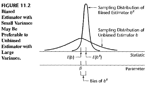
Ridge regression perturb the estimated coefficient $b_R$ from the unbiased estimator $b$, and therefore it could remedy multicollinearity problem. In other words, our unbiased estimator $b$ is obtained by the observation $X$ with multicollinearity, but slightly perturbed estimator $b_R$ is obtained by a virtual perturbed observation $X_R$ without multicollinearity. When perturbing $b_R$, we add restriction on $b_R$ to have small norm(length). Length restriction makes the variance of the sampling distribution of $b_R$ shrink. Although, $b_R$ is no longer an unbiased estimator, we have more chance to obtain $E(b_R)$ from a sampled $b_R$ compared to obtaining $E(b)=\beta$ from a sampled $b$. The relationship is given as a figure.

ridge regression

To obtain $b_R$, we consider using correlation transformed $X$ observations. This process normalizes the variable $X$ adjusting the magnitude of $SSE = (Y-X\beta)^t (Y-X\beta)$. $b_R$ can be obtained by minimizing a modified sum suquared error function $Q(\beta) = (Y-X\beta)^t (Y-X\beta) + c \beta^t \beta$ where $c$ is a given biasing coefficient and $c \leq 0$. Squared $\ell_2$ norm of $\beta$ is added in the function. This allows to minimize both $SSE$ and the length of $\beta$, at the same time. The intensity to keep focus on minimizing the length of $\beta$ can be adjusted by choosing the coefficient $c$. Larger the value $c$, the minimizing process would be more focused on minimizing the length of $\beta$. Resulting normal equation is $(X^t X + cI) b_R = X^t Y$. Therefore, $b_R = (X^tX + cI)^{-1} X^tY$.

Choice of biasing constant $c$ As the biasing constant $c$ increases, the bias of the model would be increased. But there exists a value of $c$ for which the regression estimator $b_R$ has a smaller total mean squared error $E(b^R - \beta)^2$ than the ordinary LSE $b$. But optimum value of $c$ varies from one application to another and it is unknown. Common heuristics to determine an appropriate $c$ are:

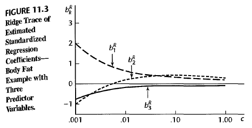
using Ridge trace Try several $c$ and plot $b_R$’s according to values of $0 \leq c \leq 1$. Take the point $c^\ast$ where the fluctuation in $b_R$ ceases.

ridge trace

using $VIF_k$ Try several $c$ and plot $VIF_k$’s according to values of $0 \leq c \leq 1$. Take the point $c^\ast$ where the fluctuation in $b_R$ ceases.

influential cases - robust regression

When an outlying influential case is not clearly erroneous, we should proceed a further examination to obtain important clues to improve the model. We may find

the omission of an important predictor variable,
incorrect functional forms, or
needs to dampen the influence of such cases.

Robust regression is an approach of regression to make the results less rely on outlying cases. There are several ways to conduct robust regression:

LAR (= LAD = minimum $\ell_1$-error) regression Least Absolute Residuals (= Least Absolute Deviations = minimum ell-one-error regression) is done by minimizing $Q_1(\beta) = \sum_{i=1}^n | Y_i - \beta_0 - \beta_1 X_{i1} - \cdots - \beta_{p-1} X_{i,p-1} |$. When there’s an outlier where its residual is large $e_i > 1$, then its squared residual gets much larger so that the regression function could overweigh this observation. This can be alleviated by using absolute values of residuals. Note that $\ell_1$ function is not differentiable. Thus, we cannot obtain an estimator $\hat{b}$ using partial derivatives. Instead, this problem can be dealt by linear programming (a kind of optimization technique).
IRLS robust regression Iteratively Reweighted Least Squares. This approach uses the weighted least square procedure as introduced before, but, weights on residuals are now determined by the magnitude of how far outlying a case is. The weights are updated iteratively in a way to flatten the weights.
LMS regression Least Median Squares. Recall that average is sensitive to outliers, but median is not. Thus, we could minimize the function $median (Y_i - \beta_0 - \beta_1 X_{i1} - \cdots - \beta_{p-1} X_{i,p-1})^2$.

2. Nonparametric regression

For complex cases, it is hard to guess a right functional form (analytic expression) of the regression function. Also, as the number of parameter increases, the space of observations gets rarefied (there are fewer cases in a neighborhood), so that the regression function tends to behave erratically. For these cases, nonparametric regression could be helpful.

regression trees

Regression tree is a powerful, yet computationally simple method of nonparametric regression. It requires virtually no assumptions, and it is simple to interpret. It is popular for explanatory studies, especially for large data sets.

regression tree

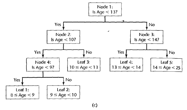
In each branch of a regression tree, the range of a specific predictor variable $X_k$ is partitioned into segments (one for $X_k \leq C$ and the other for $X_k < C$). In the terminal nodes of the tree, we evaluate the estimated regression fit by taking the mean value of the response in that segment. i.e. $\hat{Y_i} = \sum_{j=1}^{n_s} Y_j$ where $Y_j$’s belong to a segment where $i$th observation belongs to. Also, $n_s$ is the number of observations in the segment.

How to find a “best” regression tree is linked with

the number of segmented regions $r$, and
the split points $X_k$ that optimally divides the data into two sets at each branch.

The basic idea is to choose a model which minimizes the error sum of squres for the resulting regression tree. $SSE = \sum_{t_i \in T} SSE(t_i)$, where $T$ is the set of all terminal nodes, and $SSE(t_i) = \sum_{j=1}^n (Y_j - \overline{Y_{t_i}})^2$. Here, $MSE = SSE/(n-r)$) and $R^2 = 1- \frac{SSE}{SSTO}$. The number of candidate models are $r(p-1)$ where $1 \leq r \leq n$. The value of $r$ is usually chosen through validation studies as $argmin_r{MSPR}$.

3. Bootstrap confidence intervals

Above regression approaches are complex so that it is hard to estimate confidence intervals using the previous analysis on $\sigma^2(b)$ or $s^2(b)$. Instead, we can approximate confidence intervals by bootstrap method. There are many different procedures to gain bootstrap confidence intervals. One example is reflection method.

An $1-\alpha$ confidence interval of a parameter $\beta$ is $b - (b^\ast(1-\alpha/2) - b) \leq \beta \leq b + (b - b^\ast(\alpha/2))$ where $b^\ast(1-\alpha/2)$ and $b^\ast(\alpha/2)$ are obtained from bootstrap distribution. $$

RA ch11 Remedial measures